Introduction
The automatic modelling of buildings has been one of the great challenges of virtual reality, having proved its applicability in several areas. The modelling process involved in creating a 3D model of an existing building, while manual, requires significant time and effort. However, the full automation of this process, with the objective of minimum or non-existent user intervention, is almost impossible and is still a problematic issue, since it fails in achieving optimal results. It is precisely in this aspect that the method we have developed intervenes, aiming to automate as much as possible the processes involved in the creation of 3D building models from 2D floor plans and to produce those optimal results.
In this article we aspire to present a method for the expeditious reconstruction of 3D building models, from the exterior and interior structure to interior and exterior distribution of objects as well as surrounding environments. This method requires several sources of information, such as buildings’ floor plans and photographs, in order to create complete interactive 3D models that represent the house and its surroundings. It is also not limited to a digital format, with the possibility of being applied to any existing 2D plans. Several known algorithms were used and others were developed to fulfill the objective of automating as many processes as possible (e.g. extraction of textures and colours from photographs). More than a compilation of techniques, it is a new method with new techniques.
Developed for users without knowledge of architecture and graphical modelling tools, our prototype has a simple and intuitive interface and requires a low level of interaction with the user because of the many automatic features (e.g. logical distribution of furniture). The resulting outcome, i.e. the 3D models of buildings, offers a high level of detail and allows the user to navigate interactively or experience guided tours automatically created. This interesting and versatile method is applicable to areas such as architecture, video games, cinema and simulation programs, amongst others.
This paper is structured as follows. Section II presents the related field work. Section III provides a general description of the proposed method for the efficient creation of 3D house models. The techniques and algorithms used to automate some processes are identified and explained in sections IV, V and VI. In section VII we present our own software prototype named AV3D (Ambientes Virtuais 3D — 3D Virtual Environments) as well as some tests and results. Finally, section VIII concludes the article and presents proposals for future work.
Related Work
Contrary to what could be presumed, the creation of 3D building models from existing information (reconstruction) (e.g. Willmott, 2001; Dikaiakou et al., 2003; Gonçalves and Mendes, 2003; Müller et al., 2004; Silva et al., 2004; Sundstedt et al., 2004) can indeed prove to be a harder task than the generation of buildings (e.g. Parish and Müller, 2001; Greuter et al., 2003; Laycock and Day, 2003; Wonka et al., 2003; Finkenzeller et al., 2005; Martin, 2005; Müller et al., 2006a; Finkenzeller, 2008; Rodrigues et al., 2008) for which there is no existing information. The 3D representation of a building that exists or has existed in the past involves, in most cases, the use of manual methods, thus, opposing automatic methods for the generation of buildings that commonly use techniques related to Procedural Modelling (PM). However, even though PM is more often associated to the generation of new structures, it can also be used to create virtual models of structures that exist or have existed in the past (e.g. Müller et al., 2005; Müller et al., 2006a; Rodrigues et al., 2007; Rodrigues et al., 2008). Ideally, the best solution would be to combine the best of both worlds, i.e. the detail level and realism typical of the manual modelling methods and the small amount of time necessary to create a model that characterizes automatic methods.
Urban procedural modelling has been the target of numerous existing literatures. The L systems, proposed by biologist and botanist Aristid Lindenmayer, are parallel rewriting systems based on grammars consisting of sets of rules. Through these systems, complex objects can be defined by replacing parts of a simple initial object using a pre-determined set of rules. Parish and Müller (2001) generate a virtual city using L systems in the generation of roads from maps and in the division of land into lots. They also apply L systems in the generation of the final geometry of buildings.
Wonka et al. (2003) generated buildings by creating facades using split grammars (subtype of the shape grammars). Split grammars are characterized by rules of division that replace a geometric shape with several others and rules of conversion that transform one shape into another. These authors introduced the concept of control grammar, which serves the purpose of making the distribution of the various elements that constitute the facade of a building in order to meet architectural rules. They also exposed an attribute matching system used to specify high-level decisions to control the way the facades are generated. Although the generated buildings are more realistic, users must learn a complex grammar and also database rules to specify the attributes. Few years later, Müller, Wonka and others (2006b) used the knowledge from the previous mentioned work to propose a new method for addressing the problem based on a mass model technique.
In the method presented in Greuter et. al. (2003), a top down approach is used for the generation of the outer facades of a building, starting from the roof and proceeding to every floor plan until reaching the desired height. Each floor plan is constructed through the extrusion of random generated polygons submitted to scaling, rotation and merging operations. Each generated floor plan serves as the source base polygon to the next one. Lastly, the floor plans are combined with union operations.
In the work of Finkenzeller et. al. (2005) it is presented a technique for the generation of floor plans and resulting 3D geometry based on the decomposition of the architectural features of the facades. The floor plans, represented by an edge-based format, are created by composing convex 2D polygons. In this method, a subdivision process is performed to build more detailed elements such as corners, walls, doors and frames.
One common feature amongst the presented research is that these techniques are mainly designed for the generation of facades, thus, leaving aside the internal structure of buildings. Hahn et al. (2006) address this matter in real time by dividing rectangular floors corresponding to the interior of buildings into rectangular rooms and hallways. However, the representation of real buildings falls out of scope from this work because the rooms are formed randomly and there are no architectural patterns taken into account.
The interior and exterior building generation is also the focus of Martins’ approach (2005). Still, the presented results lack some realism, though it is interesting to notice that some architectural issues are taken into account. Indeed, the author (and also some of the previously mentioned literature) acknowledges the architectural patterns described in 1977 by Christopher Alexander’s in “A Pattern Language” (Alexander et al., 1977), which may serve as a basis to several architectural applications.
Rodrigues et al. present several methods based on architectural rules and laws to create virtual 3D models of houses covering the generation of modern houses (including their interiors) and the reconstruction and generation of cultural heritage structures, with applications in diverse areas such as architecture (Rodrigues et al., 2008a; Rodrigues et al., 2008b), Archaeology (Rodrigues et al., 2007; Rodrigues et al., 2008c) and virtual worlds (Rodrigues et al., 2009).
Another issue addressed in this article concerns the automatic distribution of furniture in a building’s rooms. This problem has been the focus of different approaches. In declarative modelling (Roux et al., 2004; Gaildrat, 2007; Tutenel et al., 2008), the user specifies constraints to describe the relationships between objects and is helped by semantic knowledge to generate a layout. Nevertheless, this type of systems requires user interaction and manual descriptions of the scene to layout.
In the work of Smith et al. (2001), connection areas between the objects are defined. Similarly, CAPS system (Xu et al., 2002) defines rules for each object that specify which type of objects their surface supports. However, the system takes several minutes to create reasonably complex interiors and does not support the featuring of objects on ceilings or walls.
Other techniques are used in the automatic placement of furniture. For example, natural language sentences are used to describe a scene in the WordsEye system (Coyne and Sproat, 2001). Calderon, et al. (2003) and Seversky and Yin (2006) also present approaches based on natural language to describe the object rules and relationships between objects. Still, because of the known ambiguities in natural language, these systems are not appropriate as a generic tool for object distribution in a scene, along with the fact that they only treat single individual scenes.
There are some systems resulting from research works related to the automatic/semi-automatic modelling of buildings from 2D architectural plans. Some works (So et al., 1998; Kashlev, 2008; Yee, 2008) are based exclusively on DXF formats and are designed for experienced users. These solutions have several limitations: they are based solely on plans of the DXF format; they cannot generate the exterior structure of a house; they do not detect windows; they do not support stairs to connect floors; they do not allow the application of colours or textures on walls, ceilings or floors; they do not support the distribution of interior objects in the rooms. Some other systems are based on building plans drafts (Do, 2001; Oh et al, 2004; Oh et al, 2006), yet, these have scale imprecisions and do not allow the representation of the interior of buildings.
In what concerns commercial solutions, there are many specific tools that work with both 2D and 3D models, either generic (e.g. Google Sketchup Pro, 2010, and 3D Home Architect, 2010) or specific, such as architecture related tools (e.g. AutoCAD Architecture, 2010, and VectorWorks, 2010). Despite the widespread usage of these tools, they are more targeted at architects and designers.
Likewise, there are also languages for the representation of geospatial information like the Geography Markup Language (GML) (Open Geospatial Consortium Inc., 2010); languages that enable the description of 3D shapes such as the Generative Modelling Language (Computer Graphics & Knowledge Visualization, 2010); and even more specific languages like the CityGML (Open Geospatial Consortium Inc., 2010), a GML language specialization for the visualization of architectural 3D models that requires its own specific browser.
Despite all these solutions, they hardly represent the most adequate means to achieve the desired objective of maximum process automation. Therefore, it should be intended to represent all geometrical and semantical information. This representation should be composed in a hierarchical correlated fashion that obeys to several spatial premises and that gathers all other essential requirements for the correct 3D representation of a building’s features and its surroundings. These factors stimulate the development of new methods and specialized tools such as the ones presented in this article.
Method Description
The purpose of the method addressed in this paper is the expedite creation of realistic 3D buildings and surrounding environments from a set of selected information: floor plans, photographs, room areas and organization, solar orientation, location, surroundings, amongst others. As a consequence of the automation of some processes the user has a reduced interaction level.
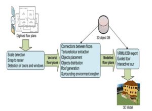
This method is very flexible and produces realistic results, needing only minimal information to create the 3D buildings. This means that it is capable of constructing a complete virtual model (exterior, interior and surroundings) while leaving a margin for perfecting the model based on the quality and quantity of the base information. Fig 1 summarizes schematically the steps required by the method to accomplish an existing building’s 3D model from a set of input data.

Fig 1. Method for the Creation of 3D Buildings
The method is decomposed in three main stages:
- Floor plan vectorization: using previously digitised plans, the scale is automatically detected so that user mistakes are avoided and the manual intervention is reduced to a minimum. Then, the user must contour every room on the floor plans with the objective of converting raster format into vectorial format. This process is assisted by a snap to raster function (snaps into image’s pixels) that augments speed and precision. An automatic process is also executed for the detection of doors and windows, taking into account the contours made by the user and also the original floor plans.
- Floor plan modeling: in the vectorial floor plans the user can now indicate the connections between each floor by placing staircases; define the types of floor, walls and ceiling, whose real colours and textures can be extracted from photos of the real rooms; place windows and doors that the automatic process did not detect; place interior and exterior objects manually or automatically; create the roofs; create the surrounding environment.
- 3D creation: finally, modelled plans and all 2D represented objects are converted into a 3D format and the guided tour paths are automatically generated. The models’ final representation is achieved through the usage of VRML/X3D technology.
The following sections present and describe all the techniques and algorithms used in the different processes of each of the stages of the 3D building creation method.
Floor Plan Vectorization
The developed method for the 3D building creation is based on its original floor plans. Taking as reference the Portuguese example, it is observed that few owners possess floor plans in digital format and many don’t even have the paper floor plans. The legal obligation of supplying digital format plans to competent authorities has only been recently imposed. If the owner does not possess the digital format plans, they will have to be obtained through requests to public entities. Currently, these entities only supply building plans in paper format. Due to these reasons and because many buildings pre-date the aforementioned legal imposition, the need to optimize the conversion of paper floor plans into digital format has become an issue.
The first stage of the method consists of the conversion of digitised floor plans into the vectorial format aided by snap to raster processes and automatic detection of doors and windows. This stage also allows the automatic scale detection.
Automatic Scale Detection
The first step of this stage consists of the automatic scale detection of the floor plans to avoid mistakes that can occur in the manual calculation process and to avoid overburdening the user with lengthy and monotonous tasks.
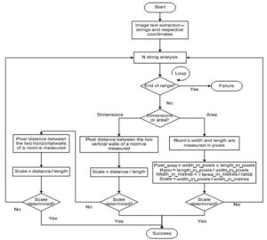
Typically, floor plans have room measures defined as length and width (i.e. metres) or as total area (i.e. square metres). So, to determine the scale, the user has to carry out some calculations. To save the time of this manual process, we have developed an algorithm — FPSE (Floor Plan Scale Extractor) — which uses OCR (Optical Character Recognition) technology to extract the impressed text from a digitised image file (raster format). All future calculations are then based on the extracted scale. The FPSE steps are described in the following flow chart:

Fig 2. Automatic Scale Detection Flow Chart
With the exception of flaws that occasionally may occur (for example, due to interferences like low quality printing in the floor plans) the method produces good results (see section VI).
Edge Detection — Snap to Raster
The initial solution to convert raster floor plans to vectorial floor plans was to use a raster-conversion tool. For this reason, we have tested several applications, such as Vector Magic (2010) and Magic Tracer (2010). Nevertheless, after several tests, we found these tools inadequate to our problem since the vast majority of existing buildings’ floor plans is still on paper format, a support prone to conditions such as low quality printing, imprecision, dirt and deterioration. In addition, many may contain small or overlapping details and confusing patterns, which prevent these tools from deciphering information in a correct way. To employ these tools, the user would have to waste a lot of time “cleaning” the original image (digitised from the paper floor plans) or correcting the final result to obtain the definitions of the rooms, windows, doors and other elements from the mass of vectors generated by the tools. This complex and time consuming task would compromise the automation level we are trying to achieve in the 3D building creation process.
Based on the performed tests, we concluded that the most effective solution would be the creation of a snap to raster function. The snap to raster is similar to the snap to grid function featured in drawing tools such as Microsoft Office Visio, but instead of performing the snap into small squares, it does so into an image’s pixels.
The objective of the snap to raster function is to make the mouse cursor, when approaching a corner formed by the floor plans’ walls, trigger the application into automatically snapping to that corner. In other words, the cursor is automatically positioned into the corner so that the user can draw the walls in a faster and more precise manner. By recognizing line midpoints, corners, intersections and line ends, this functionality enables the user to draw over a floor plans’ image.
To implement the snap to raster function we use two algorithms: one for corner detection and the other for edge detection. For the first one, we choose to use the SUSAN (Smallest Univalue Segment Assimilating Nucleus) algorithm (Smith and Brady, 1997). For the second one, we have created a new algorithm specifically for that purpose.
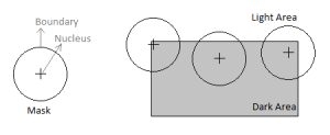
The SUSAN algorithm neither makes suppositions about the local image’s structure around a certain point nor searches for interest points (i.e. points that have a clear definition, a well-defined position in image space and are rich in terms of local information contents). Instead, it separately analyses several areas by using local direct measures and finds places where the individual region limits have a high curvature, i.e. it finds corners formed by individual areas. Thus, in bifurcations involving more than two areas (e.g. in a “T” form) where more than one single area might contribute for the detection of a corner, all the intersections will be correctly processed, no matter the complexity degree of the situation (Smith and Brady, 1997). Fig 3 shows that in an area where a corner lies a quarter of its pixels inside the circular mask called USAN (Univalue Segment Assimilating Nucleus) the pixels have identical gray scale values. For this reason, finding a corner is almost equivalent to finding a USAN which has a quarter of pixels with identical gray scale values.

Fig 3. Three Circular Masks at Different Places on an image Trying to Detect Edges
(adapted from Smith and Brady, 1997)
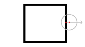
In the edge detection algorithm, an angular search is performed for each angle (with its centre at the mouse location), thus, measuring the number of adjacent pixels traversed. Then, the closest set with a number of pixels above a certain threshold is chosen. After attaining the pixel set, its centre point is calculated and used as the centre of the cursor’s closest wall. In the next figure, the red dot represents the mouse location, the red line represents the closest set of adjacent pixels and the blue line demonstrates how the set forms a line that points to the cursor.

Fig 4.Edge Detection Process
Detection of Doors and Windows
To increase the level of automation in our method, we have added a feature to automatically detect doors and windows. The algorithm created for this purpose uses a recognition technique for geometric shapes and is done in real time, as the contours of the floor plan are designed by the user. The algorithm searches for doors and windows above the contours of the image’s floor plan and it is divided in three steps described next.
Extraction of the Search Area of the Image’s Floor Plan
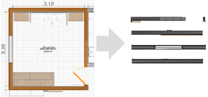
In this step, the algorithm starts by cropping the parts of the image that lie under each wall designed by the user. The new images have a length equal to the wall and a width equal to the thickness of the designed wall plus an increment of 50% tolerance. Fig 5 shows the four new images extracted from a room. If the wall drawn by the user is curved, then the part of the image extracted by the algorithm is transformed into a straight shape so that the algorithm becomes more efficient and simpler.

Fig 5. Extracted Images from the Room Walls
Detection of Potential Side Edges
The purpose of this step is to identify potential side edges of windows and doors from the extracted images in the previous step. This process consists in the detection of vertical lines with a length greater than a certain value (i.e. thickness of the wall). Since the image scale is known from the scale detection step, and the edges of the windows/doors are the joints between them and walls, the algorithm can make a first search for the vertical lines. All the vertical lines shorter than the thickness of the wall can be discarded because the edge of a window/door has a length equal to the wall. So, for each image, a search for a vertical line is performed for each X coordinate.
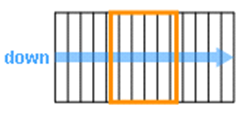
After having detected the vertical lines, a second filter has to be applied to determine those which may be potential window’s/door’s borders. A line is an edge of a window/door if it has on one side a wall and on the other a window/door, or if it has a window/door on both sides. Therefore, for each detected vertical line, the algorithm calculates for each side the percentage of the line that is in contact the x-1 and x+1 lines (see Fig 6). If at least one of the two sides has a contact percentage lower than 75%, then the vertical line is considered to be a potential edge of a window.

Fig 6. Detection of Side Edges
Determination of a Window/ Door
In this step, each pair of edges is analyzed to determine if the pair represents a window/door. For each one, horizontal lines between the edges are detected. Then, based on the information about the edges and horizontal lines, a score is calculated to determine whether or not the pair defines a window/door.
The process is done through the calculation of the percentage of pixels that fills the line for each Y coordinate. If the value is greater than 90%, then it is considered that in the current Y coordinate there is a horizontal line. In addition, the average colour of the line is also calculated. When there are adjacent horizontal lines with similar colours, then it is considered that these lines define a single thick line.
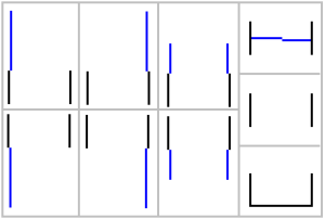
With the potential edges of a window/door and with the horizontal lines, the result of the score can be found. Through the observation of Portuguese floor plans, we have come to the conclusion that the windows are usually represented in four different ways (Fig 7) and the doors in nine ways (Fig 8 )

Fig 7. Window Types Represented in Floor Plans

Fig 8. Door Types Represented in Floor Plans
For each type of window, a score is calculated and if there is at least one type with a score greater than 90%, then the edges define a window. The scores are calculated based on the following items:
- Degree of similarity between the left and right edge, in terms of both length and positioning;
- Proximity of the horizontal lines in relation to the position where they should be;
- Image area not covered by horizontal lines.
The same goes for the calculation of the score for the doors. From the previous characteristics, the first and the third ones are also applied to the doors. In addition, the next items are also taken into consideration:
- Proximity of the horizontal lines in relation to the position where they should be and the length they should have;
- Proximity of the vertical lines in relation to the position where they should be;
- Proximity of the length of the vertical lines in relation to the distance between the left and right edges — the length of a door must equal (considering a threshold value) the distance between the edges because when the door closes, it is obvious that it must range the whole passage.
Floor Plan Modeling
The floor plan modelling stage comprises the application of the extraction processes of textures and colours, connections between floors, objects placement and distribution, roof generation and creation of surrounding environment in vectorial floor plans.
Texture Extraction
Besides the creation of the inner and outer building structure, the developed method also allows the extraction of textures from real photographs in order to enhance the realism of the final building models.
To make the texture application process easy, fast and realistic, it was necessary to develop a texture extraction process. To achieve this goal, we had to resort to a common method in image processing, that is, the detection of contours in an image. Contours in images are strong contrast intensity areas (from one pixel to the other). Contour detection procedure significantly reduces data quantity and filters useless information, thus, preserving the image’s structural properties.
The developed texture detecting technique is executed when the user needs to add new textures to apply to a wall, floor, ceiling, window, amongst others. This way, the user sees his/her work facilitated by simply passing the mouse cursor over an image to automatically discover several highlighted rectangular areas (most of the times, tiles and mosaics) in the cursor’s position.
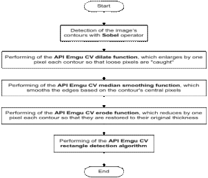
The technique applied in the automatic texture extraction uses existing algorithms. Through a specific order of the algorithms and by passing the output of one algorithm as the input of another, meaningful results are attained. This technique employs the Sobel operator (Sobel and Feldman, 1968) to detect image contours and some Emgu CV functions (a cross platform, net wrapper to the Intel OpenCV image processing library) (Emgu CV, 2010). The technique is described as follows:

Fig 9. Automatic Texture Extraction Process
The Sobel operator calculates the image intensity gradient in each point, giving the direction of the maximal possible increase from light to dark and the change rate in that direction. The result shows the abrupt or smooth changes verified in the image at that specific point, permitting to conclude whether that part of the image represents a contour and which is its orientation (Green, 2002; Matthews, 2002).
Sobel presents quite effective results in cases where the passage from one colour to another is quite strong (for example, from a blue tile to a white joint). However, when the passage is subtle (in the case of a white or light grey tile to a white joint) Sobel experiences some problems in contour recognition. Nevertheless, it presents a good tolerance to interferences, it possesses a low error rate, it is effective and it is computationally more efficient than other analyzed algorithms (for example, Prewitt, LaPlace, Canny, amongst others).
The correct preparation of an image through the use of the Sobel operator and some Emgu CV functions allowed the texture extraction technique to present very good results (see results in Fig 22).
Colour Extraction
The same way the texture extraction is important in the 3D building creation method, so is the colour extraction from a photograph. Together they represent two techniques significant in process automation, thus preventing the need of user intervention.
Taking as example a common photograph of a wall, we can observe that a wall might have undesired objects such as doors, windows, furniture, paintings, and others. Also, a wall rarely presents the same colour throughout its extension due to factors such as shadow and reflexes created by lighting, dirt, or even painting flaws. This way, we have developed a new colour extraction algorithm that takes into account the referred incidents. Nevertheless, it does not consider the fact that the photograph colours may be altered due to interior shadows or brightness from a nearby window.
The algorithm, named DBCE (Density Based Colour Extractor), searches the “centre” of the most common colour sets present in the image. Basically, the image is converted into a three-dimensional cube whose actual dimensions represent one of the RGB colour (Red, Green and Blue) components. Each cube dimension has got a 256 length that is representative of the 256 different values a colour component might have. Each small square contains a numeric value that indicates the pixel quantity of a certain colour present in the image.
For instance, if there are 120 pixels with the RGB colour 255, 0, 0 (red) in an image, the small square in the 255, 0, 0 coordinates will have a value of 120. With the 3D cube, one must only find its denser inner location and, based in a diameter 6 sphere, obtain the image’s most common colour. When searching for the denser location, it is taken into account that the larger the square value is, larger will also be its weight. Since the sphere contains the denser location, its centre will present the final colour that is the one that exists in larger quantities in the image. To illustrate the technique, we provide the following pseudo-code description:
Color DensityBasedColourExtractor (Color[][] image, Integer
imageWidth, Integer imageHeight)
{
cubeRGB = new Integer[256][256][256]
for(x=0; x<imageWidth; x++)
for(y=0; y<imageHeight; y++)
{
color = image[x][y]
cubeRGB[color.Red][color.Green][color.Blue]++
}
radius = 3
best = 0
bestColor = null
for(r=radius; r<256-radius; r++)
for(g=radius; g<256-radius; g++)
for(b=radius; b<256-radius; b++)
{
sum = 0
for(r1=r-radius; r1<r+radius; r1++)
for(g1=g-radius; g1<g+radius; g1++)
for(b1=b-radius; b1<b+radius; b1++)
sum = sum + cubeRGB[r1][g1][b1]
if(sum>best)
{
best = sum
bestColor = new Color(r,g,b)
}
}
return bestColor
}
Connections between Floors
A house or even an apartment might have several floors usually connected by stairwells which are also supported by the present method. This way, when it becomes necessary to create a connection between two floors through stairwells to allow the user to freely navigate among floors, the method takes into consideration ceiling and floor gaps in staircases’ start and end floors. The placement of staircases is done as follows:
If first step does not overlap a wall
Valid step
Select staircase type
If building possesses more than two floors
Select destination floor
Else
Remaining floor is automatically selected
Define position of the last step through the alteration of staircase length and/or width
If no overlapping situations in start and end floors between walls and staircase positions
Ladder successfully created
Once the staircase is placed, the user should insert the stairwell’s ceiling and floor dimensions so that navigation between floors is possible. The ceiling gap should always have one of its sides touching the last step of the staircases, otherwise, it will be considered invalid by the method as it can be seen in the first image of Fig 10. This is a manually conducted process because the ceiling gap dimensions are always different from case to case and do not follow a standard that could be incorporated in the method. From the moment the gap is correctly placed, the user can be assured that after the 3D model is created he/she will be able to navigate among floors.

Fig 10. Structure Opening between the Staircase’s two Floors: Invalid (left) and Valid (right).The Rectangle with the Thicker Line Represents the Ceiling Gap
Objects Placement
Besides reproducing the interior structure of the buildings, in our method it is also possible to augment the 3D models realism by placing several interior objects (like furniture, fireplaces and decoration objects) and exterior objects (such as trees, flowers, garden tables and chairs).
Interior objects have been classified according to three positioning places: floor, ceiling, and wall. In the first place are included most of the house objects: tables, sofas, beds, bathtubs and so on. Ceiling type objects include lamps, fans, amongst others. At last, wall objects include paintings, wall lamps, kitchen cupboards, and others.
Object positioning is done in 2D through the use of the information contained in a 3D object database. When rendering objects, every single one is considered according to its containing box or bounding box. This way, any object is placed as close as possible to the ceiling, wall and/or floor. A wall object, like for example a kitchen cupboard, will have marked in its entry in the database which sides of the cube can be placed against the walls and its distance from the floor, so that it can be correctly placed in the final 3D model.
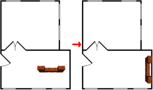
To make sure the task of object positioning is quick, the method enables to snap the object towards the nearest wall in the moment of its placement inside the room. In the example of the kitchen cupboard, its front can never be placed against a wall because its definition in the database already defines that only the back is permitted to do so. When an object features more than one of such sides, it is the closest to the wall that will be privileged or, alternatively, the side that requires the object’s minimal rotation (Fig 11).

Fig 11. Object Automatic Snap towards The Nearest Wall
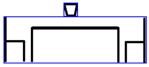
The method also allows the positioning of an object over another, meaning that it is possible to place a television on the top of a TV table. This type of object positioning had to be developed in a different way, since in some cases the objects’ bounding boxes could not be used. This is due to the fact that objects seldom result in perfect cubes. If the positioning was guided through the objects bounding boxes the outcome would be unrealistic (see left image of Fig 12).
To solve this problem, objects are decomposed into smaller parts.For example, in the right image of Fig 12,if it is intended to place a jar-object on top of the table with chairs, the jar’s bounding box is placed as near as possible to the table’s top (the object that is placed immediately below). Thus, since there are no overlapping bounding boxes or spacing, the result is correct for the human eye.

Fig 12. Wrong Jar-Object Positioning (Left) and Right Positioning (Right)
Objects Distribution
In our method, it is also possible to distribute objects automatically through the rooms of the building. Following a room by room approach because of the function specificity in each room, the created algorithm performs the furniture distribution according to placement constraints and a set of semantic rules attained from the observation of real floor plans and from common sense. The method allows the objects to be placed arbitrarily but achieving stable configurations (according to their placement constraints and semantic rules) which results in layouts of visual richness and realism.
A set of constraints is associated with each type of object to define where the object may or may not be placed. The proximity constraints type determines the minimum space that is necessary to exist between the objects. Another type of constraints defines if the top surface of an object can support other objects, or the opposite: if an object can be placed in the top surface of others.
To create realistic and coherent layouts, the distribution of objects is ruled by semantic rules including definitions for the function and fragility of objects, and for the interactions and relationships between them. The algorithm uses the already referred database of 3D objects which contains all the information necessary to the placement calculations.
When planning a logic layout, this automatic functionality also considers only the 2D bounding boxes to plan where an object is to be placed. This is due to the very complex shapes that 3D objects can have.
The method is decomposed into three steps: choosing the objects to be placed in the house, determine the objects positions according to constraints and lights placement.
Objects Selection
The objects that will be placed in a room depend on the room type and its specific set of objects. For instance, a toilet, a bathroom sink and a bathtub only appear in a bathroom. However, it does not mean that a given room will receive all the objects that it is supposed to. There may be situations where not all the objects can be placed due to insufficient space, door passage blocking, collisions between objects and opening doors, or even objects overlapping with windows.
So, the first thing that the algorithm does is to determine what object types will be placed in a given room according to its function. Randomly, the algorithm will choose the object types and quantities from each one according to a set of rules.
Then, the algorithm randomly chooses for each object type the specific object from the database to place. For performance issues, if a particular object was chosen in a room, and if the object type is repeated in another room, the same object will be chosen for this last room. This minimises the number of different objects being used in the house, therefore, reducing the size of the final model.
Objects’ Positions
For wall objects, i.e. objects intended to be placed on walls, the selection of walls where they can be placed against is done according to their length and their distance from the door of the room. So, the walls may or may not be ordered according to their distances from the door of the room.
For some rooms, priority is given to the walls where certain objects can be placed side by side (e.g. in a bathroom the priority is given to the wall that can support a bidet and a toilet). In this situation, the lengths of the objects’ bounding boxes are added along with the value of the minimum spacing between them, which is obtained according to their proximity rules. Until the algorithm finds a wall to place the objects’ sequence, the objects will keep being removed and placed on separate walls.
If an object is to be placed close to the door, then the walls where it can be placed are ordered upwardly by the distance between the centre points of the wall and door passage. On the other hand, if an object is to be placed far from the door, then the walls are ordered in descending order of distance to the doors. For an object that can be placed randomly (e.g. plants or paintings) its walls are arbitrarily ordered.
Another aspect to account for is the relationships between objects, so that the objects with no dependencies are placed first. For example, in a bathroom the sink is usually placed closest to the door, right after that the bidet is placed and finally the toilet. In this situation the toilet depends on the bidet and the bidet depends on the sink. Since the sink has no dependencies, it is the object to be placed first.
Most of the objects are placed against a wall with specific layout rules (e.g. object placed on the side of a wall closest/farthest to/from the door). For random placement objects an arbitrary position in the wall is chosen. If an object is to be placed side by side with a previously placed object, it is placed immediately after the positioned object with the appropriate spacing obtained from the proximity rule set.
Once an object is placed, its position is adjusted so it does not overlap any previously placed objects, walls or opening doors. This procedure is done by using simple geometric operations such as line intersection detection and “point in polygon” checking. Still, there may be situations where overlaps still occur. If it is the case of side by side sequences, an object is removed and placed on a separate wall. If not, either an object is switched to a smaller object type (e.g. bathtub replaced by a shower) or if it is a non-critical object, it is simply removed (e.g. a bidet). In both cases, the placement algorithm starts over.
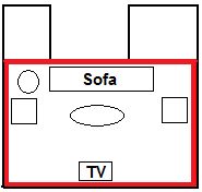
There are other situations where objects may not be placed against walls, such as dining tables or a sofa in front of a TV with no wall behind it. In this last case, to perform this type of placement, real and false walls are used by the algorithm and a set of semantic rules are used. In the sofa and TV example, to determine whether or not false walls are needed, it must first be determined if there is enough space on the existing walls where the objects may fit and at the same time if those walls are not too far from the TV. If there is not enough space using existing walls, then false walls must be calculated. False walls define a 2D bounding box that does not overlap any existing walls, so the objects cannot be placed against its edges neither too far nor too near from the TV.
When calculating the bounding box, real walls that are at the right distance to the TV and have an angle close enough to the angle of the wall where the TV is, can be used for determining the far edge of the box. If a wall is at the right distance to the TV and has an angle close enough to the perpendicular of the wall where the TV is, then it can be used for determining a lateral edge of the bounding box, as it can be seen in Fig 13

Fig 13. Created Bounding Box of False Walls (Thicker Rectangle) for the Positioning of Objects around the TV
If there are no existing walls that can be used to determine either the far edge or the lateral edge of the bounding box, then a random edge is calculated within the minimum and maximum distance to the TV.
Once the bounding box is calculated, the living room objects can be placed as if its edges were real existing walls.
Placement of Light Sources
The algorithm’s last step consists of the placement of lights throughout the rooms of the house. Lights can be placed in four different ways: against the walls, on the floor, over the furniture or against the ceiling. In the case of floor and over the furniture lights, the placement is treated as with all the other objects in the previous step.
In wall lights placement, the algorithm starts by obtaining all the walls that can receive lights (even parts of walls between windows, doors or already placed objects). Once the walls are obtained, the number of lights needed is calculated dividing the total length of original walls in the room by the maximum length of wall that a light can illuminate.
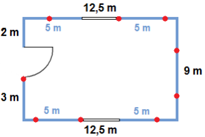
The next step is to evenly distribute the number of lights through the obtained walls. In Fig 14, an example can be seen of a room with a total original wall length of 39 metres, a usable wall length of 34 metres and where each light can illuminate a 4 meter radius. The lights are represented by red dots, the blue lines represent walls that can receive lights, the dark rectangles represent windows and the opening on the left wall represents a door. In this example, starting from the door on the left wall, the algorithm attempts to place lights at equal distance from each other (i.e. 4 metres) and when a light happens to lie on a portion of wall that can’t receive a light, the algorithm jumps to the beginning of the next valid wall and places the light there. Once the desired number of lights has been placed or the entire perimeter of the room has been traversed, the algorithm ends.

Fig 14. Placement of Wall Lights in a Room
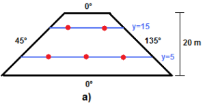
If a light is to be placed on a ceiling, the placement becomes a little more complex. First, the algorithm has to find all the different angles defined by the room’s walls (see Fig 15). Next, it rotates the room by each determined angle and for each one calculates horizontal lines that represent paths where lights can be potentially placed. These lines have to be placed in a way that allows the room to be completely illuminated and at the same time with the least amount of lights. Therefore, the lines will have to be placed as far apart as possible with a spacing no greater than the diameter of illumination of the lights to place. To achieve the correct number of lines and their positions, the following calculations are made:
- number_of_lines = Round up (rotated_room’s_height / diameter_of_illumination)
- new_diameter_of_illumination = rotated_room’s_height / number_of_lines
- Place the first line at: y = new_diameter_of_illumination / 2
- Place remaining lines at: distance of new_diameter_of_illumination from the previous line.
For each calculated horizontal line, the portions contained inside the room are calculated using line intersection equations. After that, for each line segment the length is calculated, then divided by the diameter of illumination and finally rounded up to determine the necessary number of lights. The lights can then be evenly distributed along the line segment. For example, in Fig 15 a) the room’s height is 20 m and the diameter of illumination of each light is 12 m. The following calculations can be done:
- number_of_lines = Round up (20 / 12) = 2
- new_diameter_of_illumination = 20 / 2 = 10
- Place the first line at: y = 10 / 2 = 5
- Place remaining lines at: y = 5 + 10 = 15
For each light, a verification is also made to determine if there are already any lights in the vicinity with a distance less than or equal to the radius of illumination. If such a light exists, then the current light isn’t placed. This process is done for each line segment and for each different angle earlier determined, because there may be situations where the simple distribution of lights in the room may produce regions without illumination due to the shape of the room (see Fig 15 b).

Fig 15. Light Ceiling Positioning (a) Trapezium Shaped Room (b) Cross Shaped Room
Roof Generation
Roofs can be extremely complex building features. For example, in a two floor house, there might be roofs other than the main one on the top floor, like some kind of roof protecting the entrances of the house. Moreover, the roof might just be flat or have some different heights, and might have curves or slopes.
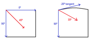
In this method, roof generation uses the Straight Skeleton algorithm presented by Felkel and Obdrzálek (1998). The Straight Skeleton algorithm enables the generation of hip roof types in straight walls’ buildings. However, some alterations were conducted so that it would become possible to extend it to the creation of roofs for buildings with curved walls. This way, and because there is a range of different real roofs, these alterations contributed to increase the buildings’ realism.
In a practical level, the modified algorithm, besides calculating the straight skeleton for straight polygons, can also carry through the calculations for curved polygons. For a certain corner, the straight skeleton calculates the angles of the two straight lines. The result is the medium value of the two. In the case of a corner composed by a straight line and a curved one, the angle of the latter is determined by its vertex tangent. So, every time the algorithm finds a curve in the roof’s polygon, it calculates the straight line tangent to the curved line in the vertex and uses it as if it was the roof’s straight line. The following results are achieved:

Fig 16. Modified Straight Skeleton Algorithm Calculations for Straight and Curved Lines
Surrounding Environment Creation
The creation of houses’ surrounding environments consists in the definition of terrain areas, placement of exterior objects and setting the view that the observer will see when looking out to the horizon of the final 3D model.
The creation of the terrain is done by defining 2D polygons that represent land areas. For example, one polygon could represent a grass area and another polygon could represent a concrete driveway. In addition, global slopes can be applied to the areas.
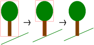
Next, objects such as trees, flowers, picnic tables and so on, can be set on the areas. An exterior object can have one of two types of placement: flat against the ground or placed vertically. In the first type, if the land has an inclination, the object will also be inclined so that it continues flat against the ground. In the second type, the object is placed vertically, no matter what the land’s inclination is, so that a tree, for example, does not tip. For this type of placement, an algorithm must be applied to determine the objects’ correct altitude at the same time that it ensures that it will not float above the ground in the final 3D model (see first image of Fig 17). To achieve these results, the object’s bounding boxes are decomposed into smaller parts, just like the positioning of interior objects above others. In the second image of Fig 17, the tree is divided in two parts: treetop and trunk. Then, the geometry of the lowest part of the object, i.e. the one that comes in contact with the ground, will be used to determine the object’s final altitude ensuring that no part of the object will float above the ground. In the third image of Fig 17, the trunk’s geometry is used to achieve the correct positioning.

Fig 17. Tree Placement in A Sloping Terrain
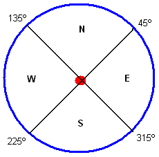
Finally, the creation of the horizon view that will be visible in the 3D final model consists in setting a panoramic image that is wrapped around the exterior of the building, as if one placed a cylinder surrounding the building with a 360º image placed in the inside of the cylinder. There are two different methods to apply the panorama in the model. In the first one, a single image is wrapped around the entire exterior of the building and, in the second, four different images are used with each one being visible to the observer depending on the direction where he/she is looking. In this second method, each image, corresponding to the North, East, South and West views, will be placed in a half cylinder. Fig 18 indicates what image is shown according to the observer’s orientation. For example, if the orientation is between 45 and 135 degrees, the North image is shown.

Fig 18. Panorama Orientation Degrees
3D Creation
The last step of our method consists of the building’s 3D creation. The final 3D models were represented using VRML/X3D technology. The next sections describe the process in detail starting from the generation of 3D geometry up to the automatic creation of tour paths.
3D Geometry Generation
3D geometry is achieved in three steps. First, walls are raised from the floor plan. Then, doors and windows are created and house objects (e.g. furniture) are added. Also, the exterior objects of the surrounding environment are added in this step. Finally, roofs are also created and added to the final model along with the panorama view.
When creating the walls a 2D polygon is generated with the defined length and height for each of the edges of the exterior walls’ floor plans. For the interior walls, each room of the house is browsed and for each one all edges are accounted for in order to create the polygons that compose the inner building’s walls. After the walls are parsed, floor and ceiling planes are also added, one for each room. In addition, the terrain areas are also added to the surrounding environment of the house.
In the second step, the integration of doors and windows starts with the subtraction of rectangles from inner and outer walls in the respective places represented in the floor plans. After the holes are made, these are filled with the geometry of corresponding doors and windows. Both windows and doors can be of three types: surrounding frame, bottom frame or frameless. For the surrounding frame, the 3D creation process applies a frame to all edges; for the bottom frame, a frame is applied only to the bottom edge; as for the last type, no frame is applied.
The addition of objects to the model is done using a database with 3D objects in VRML/X3D format. This object database was previously used in the object distribution stage for the choice of the objects to distribute in the floor plan.
The algorithm used in the third step, taking into account the 2D layout plan, searches the VRML/X3D 3D object database to find each necessary object. The algorithm uses 3D bounding boxes and makes all the scale modifications that may be needed for the objects to fit in the appropriated place. After that, all 3D objects are placed in the correct locations. However, in the case of interior objects that need to be placed in top of others, these have to be decomposed in smaller objects to determine the vertical positioning.
Finally, in the last stage, the roof structure and the panorama view are added. First, all edges of the roof are created according to the 2D floor plan. Then, the remaining roof is created by following a straight skeleton approach. Lastly, to enhance the realism of the roofs, 3D half-cylinders are placed on each of the straight skeleton edges to represent the roof spines. 360º images are also placed around the building and added to the final model.
After the execution of all previous stages, the geometry is modelled into VRML or X3D. Both technologies allow the visualization of all elements of the building (exterior, interior and surroundings components) through a 3D perspective where the user can navigate through the exterior and interior of it. To increase the realism of the scene, the generated models also include collision detection, proximity sensors for turning on lights and opening/closing doors.
Calculation of the Guided Tour Path
The 3D models created by our method offer two types of interaction: manual or automatic. In the first type, the visitor can freely explore the building, both exteriorly and interiorly, through the usage of keyboard and mouse. In the automatic interaction, i.e. guided tour, the users can visit the entire building without having to learn how to operate with VRML/X3D viewers. The visitors watch a guiding film that takes them through the exterior and into the interior rooms. This last interaction kind is achieved through paths automatically pre-calculated when the 3D model creation was being concluded.
To calculate the guided tour’s automatic path through the 3D building we have created the algorithm named FPPC (Floor Plan Path Calculator). FPPC is based on the A* algorithm (Hart et al, 1968), which is one of the most popular and flexible algorithms used in the path search problem resolution, from a start point to an objective-point, avoiding obstacles and minimizing computation costs.
The A* algorithm is a combination of two others: the Dijkstra algorithm (Dijkstra, 1959), used to find the shortest path, and the Best First Search (BFS) (Pearl, 1984), which is guided by a heuristic. The success of the A* algorithm lies in the combination of pieces of information used by Dijkstra, such as the privileging of vertexes closer to the departure point, and others used by the BFS, namely the privileging of vertexes closer to the objective.
The FPPC algorithm applied in the guided tour is based on the shortest and simplest path calculations of A*, but with some modifications. It uses a predetermined room as a start point and another as an objective point. Because in the A* the touring area must be converted in squared space where each small square is marked as areas that can or cannot be crossed, the result is a set of small squares that define the ones that have to be crossed from the start point to the end point. Considering that the house is a continual space and not a discrete one, the A* results are worked in optimizing fashion, avoiding abrupt direction changes, typically vertical, horizontal and diagonal paths and others (see Fig 19).

Fig 19. Results and Optimisation of the A* Algorithm Path
As a result, the trajectory of the 3D building that the user sees is the best-path calculated with the objective of tour optimization.
Tests and Results
This section presents the results of some of the used techniques, AV3D — the developed software prototype to test the method — and some images with 3D final models produced with AV3D. The results presented in this section and in the last one were obtained on a system equipped with an Intel Core 2 Duo at 2.67GHz with 4 GB of RAM. However, minimum requirements for AV3D can be provided by a system equipped with an Intel Pentium 4 at 1.3 GHz with 2 GB of RAM.
Used Techniques
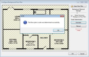
The automatic detection of the floor plan’s scale is realized by the user through the opening of the floor plan by simply clicking on the Estimate Scale button. Rapidly, the application shows the result of a 47 pixels scale, as it can be seen in
Fig 20.

Fig 20. Automatic Scale Detection Calculation Results
In the previous figure, the lounge room has a 5.0m width and a 235 pixels distance between walls. Dividing 235 by 5 we obtain the 47 pixels per metre scale. If the strings were defined in square metres and not in metres, and the lounge room had a 17 square metres area, the calculations would be as follows:
- width_in_metres = √ (17 / 0,68) = 5 m
- scale = 235 / 5 = 47 pixels per metre
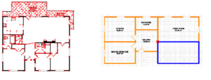
SUSAN’s effectiveness in vertex detection, shown in the first image of Fig 21 where the detected vertexes are highlighted, enabled its integration in our method for the automation process of 3D buildings’ creation. The result of its application in the AV3D prototype is shown in the second image of the same figure, where the little square represents the automatic snap vertex resulting from the merging of the two rooms. The user places the cursor next to a vertex and if the method considers that the room can be closed, a new wall is automatically placed, highlighting the room blue, thus, preventing errors and facilitating the process.

Fig 21. Results of The SUSAN Testing and Prototype Implementation
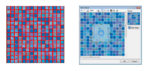
The effectiveness of the application of the Sobel contour detection algorithm and its work with several API Emgu CV functions could be tested and implemented in our prototype as is shown in Fig 22. In the first image, detected contours are highlighted in red. In the second image, corresponding to the extraction of a texture feature in AV3D, the user has simply passed the mouse over the image, thus causing the pattern’s automatic selection.

Fig 22. Sobel Test Results and Prototype Implementation
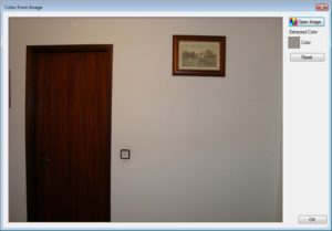
The next figure reveals an image of our prototype extracting the predominant wall colour of the photograph. The user, by opening the photograph, can immediately contemplate the automatically extracted colour.

Fig 23. Results of the Prototype’s Colour Extraction Process
These results represent only a small part of the several tests that were conducted in the process creation of the method.
AV3D Prototype
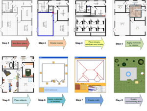
AV3D is divided into steps, which correspond to different objectives, so that the user can efficiently use it. Several complete house models were produced with AV3D, and after a few tests with some subjects who have never used the application, the results show that users, after only a few models, tended to significantly reduce the amount of time necessary to produce a complete visual appealing traversable house. Fig 24 shows the results of the several steps of AV3D.

Fig 24. Results of Each Step of the AV3D Prototype

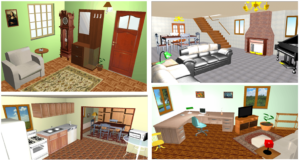
Fig 25. Building Interiors

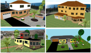
Fig 26. Building Exteriors
Interior and Exterior Results
Finally, figures Fig 25 andFig 26, show several screenshots of a variety of modelled building’s interior and exterior.
Conclusions and Future Work
In this paper, we have presented a method for the expedite creation of realistic 3D buildings’ virtual environments from a set of selected information (e.g. floor plans, photographs, amongst others). The method is capable of constructing a complete virtual model (exterior, interior and surroundings), leaving a margin for the perfecting of the model based on the quality and quantity of the base information. As a consequence of the automation of some processes that will always guarantee good results regardless of the specificity of the situation, the user has a reduced interaction level.
We also introduced our AV3D prototype, which implements the developed method, to show the simple steps that a user has to make to create a 3D building in a matter of minutes (about 10 to 15 minutes). On every step, the user can apply several automatic features to facilitate the task and has the possibility to add more details. The automatic distribution of objects feature is also noteworthy. As we have seen in the related work section, there are some methods that try to solve this problem. However, they always present some kind of constraints to our desired purposes. For this reason, we developed an algorithm that works very well for our main objective: logical distribution of objects in rooms in less than 3 seconds.
Summarizing, our method presents several advantages: it is targeted for users without expertise in architecture or computer graphics apart from other similar programs; it is not limited to a digital format, it covers most of the existing 2D plans; in addition to the creation of a building it also creates the surrounding environment; it allows the extraction of textures and colours from real photographs; the developed prototype has a simple and intuitive interface decomposed in 9 steps.
Being such a flexible and realistic method, it can be applied to many different areas: architecture, virtual games, cinema, simulation programs, amongst others. Obviously, for each of these different areas, the method would have to be adapted and optimized in order to fit specific requisites.
In the future, with the prospect of the method being able to work directly with vector formats (such as DWG), new approaches that allow a higher level of automation will be explored, thus, greatly reducing the work done by the user. This is also the case with automatic recognition of floors. We also want to cover more architectural elements, such as the ones currently existing in contemporary architecture houses (balconies inside the buildings, rooms with the height of two floors, etc.). Additionally, we will develop a 3D editor to replace the current 2D editor, since it will allow a more realistic perspective during all the steps of building creation.
Acknowledgment
The research described in this paper has been partially funded by the National Strategic Reference Framework (NSRF) which constitutes the framing for the application of the Community’s policy for economic and social cohesion in Portugal for the 2007-2013 period.
References
3D Home Architect, [Retrieved 15 June, 2010], http://www.3dhaonline.com/
Publisher
Alexander, C., Ishikawa, S. and Silverstein, M. (1977). “A Pattern Language,” Oxford University Press, New York.
Publisher – Google Scholar
AutoCAD Architecture, [Retrieved 15 June, 2010], http://usa.autodesk.com/
Calderon, C., Cavazza, M. & Diaz, D. (2003). “A New Approach to the Interactive Resolution of Configuration Problems in Virtual Environments,” Proceedings of the 3rd International conference on Smart Graphics, 2-4 July 2003, Heidelberg, Germany.
Publisher – Google Scholar – British Library Direct
Computer Graphics & Knowledge Visualization, Generative Modeling Language, [Online], [Retrieved 15 June, 2010],http://www.generative-modeling.org/
Coyne, B. & Sproat, R. (2001). “WordsEye: an Automatic Text-to-Scene Conversion System”, Proceedings of International Conference on Computer Graphics and Interactive Technologies (SIGGRAPH 2001). Los Angeles, California, USA, 487-496.
Publisher – Google Scholar
Dijkstra, E. W. (1959). A Note on Two Problems in Connexion with Graphs, Numerische Mathematik, 1, 269—271.
Publisher – Google Scholar
Dikaiakou, M., Efthymiou, A. & Chrysanthou, Y. (2003). “Modelling the Walled City of Nicosia,” Proceedings of the Virtual Reality, Archaeology, and Intelligent Cultural Heritage 2003 (VAST). 2003, Brighton, United Kingdom, 57—65.
Publisher – Google Scholar
Do, I. & Yi, E, (2001). “VR Sketchpad — Create Instant 3D Worlds by Sketching on Transparent Window,” CAAD Futures, Vries, B., Leeuwen, J., Achten, H. (Eds.). Kluwer Academic Publishers, 161-172.
Publisher
Emgu CV, [Retrieved 15 June, 2010], http://www.emgu.com
Felkel, P. & Obdrzalek, S. (1998). “Straight Skeleton Implementation,” Proceedings of Spring Conference on Computer Graphics, Budmerice, Slovakia, 210-218.
Publisher – Google Scholar
Finkenzeller, D. (2008). “Detailed Building Facades,” IEEE Computer Graphics and Applications, 28, 58-66.
Publisher – Google Scholar – British Library Direct
Finkenzeller, D., Bender, J. & Schmitt, A. (2005). “Feature-based Decomposition of Façades,” Proceedings of Virtual Concept, 2005, Biarritz, France.
Publisher – Google Scholar
Gaildrat, V. (2007). “Declarative Modelling of Virtual Environments, Overview of issues and Applications,” International Conference on Computer Graphics and Artificial Intelligence (3IA 2007). 30-31 May 2007, Athens, Greece.
Publisher – Google Scholar
Gonçalves, A. J. M. & Mendes, A. J. (2003). “The Rebirth of A Roman Forum: The Case Study of the Flavian Forum of Conimbriga,” Proceedings of Enter the Past – The E-way into the four Dimensions of Cultural Heritage Congress, April 2003, Wien, Austria.
Publisher – Google Scholar
Google Sketchup, [Retrieved 15 June, 2010], http://sketchup.google.com/
Green, B. (2002). “Edge Detection Tutorial,” [Retrieved November 3, 2009],
http://www.pages.drexel.edu/~weg22/edge.html
Greuter, S., Parker, J., Stewart, N. & Leach, G. (2003). “Real-time Procedural Generation of ‘Pseudo Infinite’ Cities,” Proceedings of the 1st International Conference on Computer Graphics and Interactive Techniques in Australasia and South East Asia, 11-14 February 2003, Melbourne, Australia.
Publisher – Google Scholar
Hahn, E., Bose, P. & Whitehead, A. (2006). “Persistent Realtime Building Interior Generation,” Proceedings of the ACM SIGGRAPH Symposium on Videogames, ACM Press, 179-186.
Publisher – Google Scholar
Hart, P. E., Nilsson, N. J. & Raphael, B. (1968). “A Formal Basis for the Heuristic Determination of Minimum Cost Paths,” IEEE Transactions on Systems Science and Cybernetics SSC4, 4(2). 100—107.
Publisher – Google Scholar
Kashlev, D. (2008). “Efficient 3D Building Model Generation from 2D Floor Plans,” Master’s Thesis, Department of Electrical Engineering and Computer Science, Massachusetts Institute of Technology.
Publisher – Google Scholar
Laycock, R. G. & Day, A. M. (2003). “Automatically Generating Large Urban Environments Based on the Footprint Data of Buildings,” Proceedings of the 8th ACM Symposium on Solid Modeling and Applications, 16-20 June 2003, Seattle, Washington, USA.
Publisher – Google Scholar
Magic Tracer, [Retrieved 15 June, 2010], http://www.magictracer.com/
Martin, J. (2005). “Algorithmic Beauty of Buildings Methods for Procedural Building Generation,” Honors Thesis, Trinity University, San Antonio, Texas, USA.
Publisher – Google Scholar
Matthews, J. (2002). “An Introduction to Edge Detection: The Sobel Edge Detector,” Generation 5, [Online], [Retrieved November 3, 2009],
http://www.generation5.org/content/2002/im01.asp
Müller, P., Vereenooghe, T., Ulmer, A. & Gool, L. (2005). “Automatic Reconstruction of Roman Housing Architecture,” Proceedings of the International Workshop on Recording, Modeling and Visualization of Cultural Heritage, 22-27 May 2005, Ascona, Switzerland, 287-297.
Publisher – Google Scholar
Müller, P., Vereenooghe, T., Vergauwen, M., Gool, L. V. & Waelkens, M. (2004). “Photo-Realistic and Detailed 3D Modeling: The Antonine Nymphaeum at Sagalassos (Turkey),” Proceedings of the XXXII Computer Applications and Quantitative Methods to Archaeology Conference (CAA). April 2004, Prato, Italy.
Publisher – Google Scholar
Müller, P., Vereenooghe, T., Wonka, P., Paap, I. & Gool, L. (2006a). “Procedural 3D Reconstruction of Puuc Buildings in Xkipche,” Eurographics Symposium on Virtual Reality, Archaeology and Cultural Heritage, 139-146.
Publisher – Google Scholar
Müller, P., Wonka, P., Haegler, S., Ulmer, A. & Gool, L. V. (2006b). “Procedural Modeling of Buildings,” ACM Transactions on Graphics, 25, 614-623.
Publisher – Google Scholar – British Library Direct
Oh, J., Stuerzlinger, W. & Danahy, J. (2006). “SESAME: towards Better 3D Conceptual Design Systems,” Proceedings of the 6th conference on Designing Interactive systems, University Park, USA, 80-89.
Publisher – Google Scholar
Oh, Y., Gross, M. D. & Do, E. Y.-L. (2004). “Critiquing Freehand Sketching — A Computational Tool for Design Evaluation,” Proceedings of the Third International Conference on Visual and Spatial Reasoning in Design, MIT, Cambridge, USA, 127-133.
Publisher – Google Scholar
Open Geospatial Consortium, Inc., CityGML, [Retrieved 15 June, 2010],http://www.opengeospatial.org/standards/citygml
Open Geospatial Consortium, Inc., Geography Markup Language, [Retrieved 15 June, 2010],http://www.opengeospatial.org/standards/gml
Parish, Y. I. H. & Müller, P. (2001). “Procedural Modeling of Cities,” Proceedings of the 28th Annual Conference onComputer Graphics and Interactive Techniques, 2001, 301-308.
Publisher – Google Scholar
Pearl, J. (1984). Heuristics: Intelligent Search Strategies for Computer Problem Solving, Addison-Wesley, 48.
Publisher – Google Scholar
Rodrigues, N., Dionísio, M., Gonçalves, A., Magalhães, L. G., Moura, J. P. & Chalmers, A. (2008a). “Incorporating Legal Rules on Procedural House Generation,” Proceedings of the Spring Conference on Computer Graphics, 21-23 April 2008, Bratislava, Slovakia.
Publisher – Google Scholar
Rodrigues, N., Dionísio, M., Gonçalves, A., Magalhães, L., Moura, J. & Chalmers, A. (2008b). Rule-based Generation of Houses, Computer Graphics & Geometry, 10(2). 49-65,
http://cgg-journal.com/2008-2/
Publisher – Google Scholar
Rodrigues, N., Magalhães, L., Moura, J. & Chalmers, A. (2007). “Geração Automática de Estruturas Romanas,”Congresso CAA Portugal 2007, 15-16 November 2007, Leiria, Portugal.
Rodrigues, N., Magalhães, L., Moura, J. & Chalmers, A. (2008c). “Automatic Reconstruction of Virtual Heritage Sites,”Eurographics Symposium on Virtual Reality, Archaeology and Cultural Heritage, 2-5 December 2008, Braga, Portugal.
Rodrigues, N., Magalhães, L., Moura, J., Chalmers, A., Santos, F. & Morgado, L. (2009). “ArchHouseGenerator – A Framework for House Generation,” Proceedings of the Slactions 2009 International Conference – Life, imagination, and work using metaverse platforms, 24-26 September 2009.
Roux, O. L., Gaildrat, V., & Caubet, R. (2004). “Constraint Satisfaction Techniques for the Generation Phase in Declarative Modeling,”
Publisher – Google Scholar
Sarfraz, M. (Ed.). Geometric Modeling: Techniques, Applications, Systems and Tools, Kluwer Academic Publishers Norwell, MA, USA, 194-215.
Publisher – Google Scholar
Seversky, L. M. & Yin, L. (2006). “Real-time automatic 3d scene generation from natural language voice and text descriptions,” Proceedings of the 14th annual ACM international conference on Multimedia, 23-27 October 2006, New York, USA.
Publisher – Google Scholar
Silva, F., Rodrigues, D. & Gonçalves, A. (2004). “House of the Skeletons – A Virtual Way,” Proceedings of the XXXII Computer Applications and Quantitative Methods to Archaeology Conference (CAA). April 2004, Prato, Italy.
Google Scholar
Smith, G., Salzman, T. & Stuerzlinger, W. (2001). “3D Scene Manipulation with 2D Devices and Constraints,” Graphics Interface Proceedings 2001, Ottawa, Ontario, Canada, 135-142.
Publisher – Google Scholar – British Library Direct
Smith, S. M. & Brady, J. M. (1997). SUSAN — A New Approach to Low Level Image Processing, International Journal of Computer Vision, 23(1). 45-78.
Publisher – Google Scholar – British Library Direct
So, C., Baciu, G. & Sun, H. (1998). “Reconstruction of 3D Virtual Buildings from 2D Architectural Floor Plans,”Proceedings of the ACM symposium on Virtual reality software and technology, 2-5 November 1998, Taipei, Taiwan, 17-23.
Publisher – Google Scholar
Sobel, I. & Feldman, G. (1968). “A 3×3 Isotropic Gradient Operator for Image Processing,” unpublished, presented at a talk at the Stanford Artificial Project in 1968.
Google Scholar
Sundstedt, V., Chalmers, A. & Martinez, P. (2004). “High Fidelity Reconstruction of the Ancient Egyptian Temple of Kalabsha,” Proceedings of the 3rd International Conference on Computer Graphics, Virtual Reality, Visualisation and Interaction, 2004, Stellenbosch, South Africa, 107-113.
Publisher – Google Scholar
Tutenel, T., Bidarra, R., Smelik, R. M. & De Kraker, K. J. (2009). “Rule-based Layout Solving and its Application to Procedural Interior Generation,” Proceedings of the CASA workshop on 3D advanced media in gaming and simulation (3AMIGAS). 16 June 2009, Amsterdam, The Netherlands.
Publisher – Google Scholar
Vector Magic, [Retrieved 15 June, 2010],
http://vectormagic.com/home
Vectorworks, [Retrieved 15 June, 2010],
http://www.nemetschek.net/
Willmott, J., Wright, L. I., Arnold, D. B. & Day, A. M. (2001). “Rendering of Large and Complex Urban Environments for Real Time Heritage Reconstructions,” Proceedings of the 2001 Conference on Virtual Reality, Archaeology, and Cultural Heritage, 2001, Glyfada, Greece.
Publisher – Google Scholar
Wonka, P., Wimmer, M., Sillion, F. & Ribarsky, W. (2003). “Instant Architecture,” ACM Transactions on Graphics, 22(3). 669-677.
Publisher – Google Scholar – British Library Direct
Xu, K., Stewart, J. & Fiume, E. (2002). “Constraint-Based Automatic Placement for Scene Composition,” Graphics Interface Proceedings 2002, May 2002, University of Calgary, 25-34.
Publisher – Google Scholar – British Library Direct
Yeung, W. Y. (2008). “Creation of 3D Model from 2D Floor Plan,” Final Year Project Report 2007-2008, Department of Computer Science, City University of Hong Kong.
Publisher – Google Scholar


