Resilience Analysis of the 2008 Economic Crisis Using Entropic Measures

Introduction

The use of predictors based on the calculation of entropy has been already tested in many economic studies. However, only few studies exist in the area of analysis of the economic resilience. The prediction of the impact of the economic crisis on the region will always be a topical issue. Employment is one of the key macroeconomic indicators and we, therefore, attach great importance to its analysis. Quantifying entropy as a measure of uniformity in distribution of economic activities in the region is a suitable predictor because it is influencable (e.g. in the form of subsidies for a certain economic activity, etc.). This paper aims to evaluate the importance of indicators based on the calculation of entropy derived from regional employment in the main economic activities in terms of predictors of regional economic resilience. Main research question is whether the higher diversity of regional employment (among economic activities) makes a region more resilient against shocks and, thus, could weaken the effects of a shock. To achieve this goal, labour dynamics of 186 regions of 11 EU Member States have been reviewed in the context of the economic crisis in 2008. These countries were selected mainly for the purpose of the geographical and historical diversity (three countries were from West, four are from South and four are form East Europe). The research question of this paper is whether entropy measures are significant predictors of regional recession (measured by employment).

Within the analytical part of the article, we estimate the β coefficients of regression analysis that indicate the importance and role of examined predictors based on the entropy calculation. The results of the statistical analysis show that the Shannon entropy and Tsallis entropy are more suitable for prediction of size of employment downturn (recession index) while the Rényi entropy is the dominant predictor of rate of employment downturn in recession phase. The results of the statistical analysis show that when Shannon entropy was growing through the recovery phase before the crisis, regions experience a higher rate of employment decrease in the following recession period. On the other hand, the higher the Shannon entropy is, the smaller the recession index is. However, the Tsallis entropy plays a different role in comparison to Shannon entropy. The higher the measured Tsallis entropy was, the more significantly the region was affected. In conclusion, the use of entropy as a resilience indicator in terms of regional policy is a significant predictor of regional resilience.

The article shows how the level of regional employment entropy determines the level of regional economic resilience (measured through the lens of the employment dynamics in main sectors). The analytical part also presents evidence to support three research hypotheses that describe the relationship between three entropy indicators (Shannon, Rényi and Tsallis entropy) and four examined resilience indicators. The methodological part describes the approach by Ron Martin (Martin, 2012) who has developed the procedure for measuring regional economic resilience. We adopt his approach in this paper.

Regional Resilience

Since the 1970s, the study of the resilience of socio-ecological systems has been the topic of many investigations. At the beginning of the 21st century, some regional economists use this concept in relation to the dynamics of the region’s economy, claiming that viewing the region through resilience prism can help explain how these systems respond to various perturbations (see e.g. Reggiani (Reggiani, De Graaff, & Nijkamp, 2002)).

The first fundamental definitions were presented by Holling (Holling, 1973) and Perrings (Perrings, 1998). For example, Hill et al (Hill, Wial, & Wolman, 2008) describe the definition of economic resilience as the ability of the region’s economy to recover from a perturbation that had a negative impact on the region’s development. Rose (Rose, 2009) sees resilience as the ability to absorb the influence of external shocks. The economic resilience of the regions to the national and international economic crises is often mentioned in the European Union since the beginning of the global economic crisis in 2008. The usefulness of understanding the factors behind the regional resilience phenomena is justifiable by the fact that the impact of the global economic crisis on the economic situation of the EU regions was asymmetrical.

On the other hand, a number of regions continue to suffer economic downturns or have been hit by a second wave of economic downturn after a relatively short recovery. The quick and successful recovery of the economies of some regions raises the question of what is behind this success. Moreover, a comprehensive assessment and synthesis of what makes some regions more resilient than others, and what regional policy makers can do to increase the resilience of the regions to the future economic crises, need to be answered.

There are three ways of seeing the economic resilience of the regions. The first is based on the so-called “engineering” concept of resilience (Modica & Reggiani, 2015). An essential characteristic of this approach is to assess the ability of the region to “go back” to its original state before crisis. For example, it may be a return of the growth rate of employment in the region to the same level before the crisis.

Within this approach, the economic resilience of the region is quantified according to the level of recovery of the selected indicator of the corresponding state before the economic downturn of the economy. The rate of economic downturn or recovery is usually measured in relation to the dynamics of regional employment or regional product, either in terms of achieving absolute value or even in terms of renewing the rate of growth of these quantities.

This approach is easily applicable and is used in studies of British economist and geographer Ron Martin (e.g. (Martin, 2012), (Martin, Sunley, Gardiner, & Tyler, 2016)). Within this engineering approach, it is also possible to evaluate the time of returning to the level before the negative economic downturn. Other suitable indicators for quantifying economic resilience index can be based on, for example, employment by industry, labour productivity, the number of workers, employment rate, economic activity rate, gross value added, the number of enterprises in the region or the number of enterprises in export sectors (Martin, 2012).

The second approach to regional resilience is the so-called “ecological” concept that emphasises the magnitude of the disturbance that the region is able to absorb before it deviates from the original state. As Walker et al (Walker et al., 2002) states, an emphasis is placed on the behaviour of the system beyond equilibrium. The resilient region has the ability to absorb the deviation from equilibrium by changing its internal structure. The purpose of this adaptation is to preserve the function of the system.

The two approaches mentioned above are criticised because, according to some authors ((Pike, Dawley, & Tomaney, 2010), (Martin & Sunley, 2007)), they do not sufficiently address the economic development perspective over the long term, which is inconsistent with the perceived dynamics of successful economies. This resulted in the third approach called “adaptive”, also known as “evolutionary” approach. This third approach highlights the ability of the system to undergo, either in a preventive way or in response to a sudden change, the modification of its structure or function to minimise the impact of destabilising change. The supporters of this approach highlight the adaptive capability of the system. They understand the region as a “complex adaptive system” that can never be in balance, and therefore the economic resilience of the region is achieved by a constant change in the region’s economy. Resilience turns into the continuous ability to adjust to stress, and the analysis of resilience becomes the study of how economics adjusts to varying stages in economic cycles (Pendall, Foster, & Cowell, 2009).

It should be stated that a change in the internal structure of the economy might not necessarily be desirable. In connection with regional resilience, the so-called hysteresis in the labour market is often mentioned (e.g. (Martin, 2012)). This is a situation where the economic downturn leads to a steady increase of the natural rate of unemployment. This negative hysteresis effect in the labour market occurs when the economic downturn is strong enough to cause a change in the behaviour of economic subjects and change the structure of the economy, thus, adversely affecting the course of the adaptive process of the region’s economy.

However, some authors believe that crises can lead to the transformation of economies towards an economic structure that is in line with the idea of sustainable development (e.g. see (Folke, Colding, & Berkes, 2003), (Duit, Galaz, Eckerberg, & Ebbesson, 2010), (Shaw, 2012)). The crisis can cause or permit the necessary transformation of economic systems ((Pike et al., 2010)).

This understanding is related to the Schumpeter concept of “creative destruction”. From this point of view, the mechanism of the positive impact of the crisis is perceived by the fact that the crisis removes those kinds of economic activities that can be considered less productive. Removing non-productive activities will create space for new opportunities for the development of new industries (Simmie & Martin, 2010).

Data, Methods and the Model

For the purpose of verifying the research question, it was necessary to implement the following preparatory steps:

1. Obtain and treat employment data from selected EU Member States.
2. From pre-crisis data, quantify predictors based on selected entropy measures.
3. From the post-crisis data, quantify the appropriate dependent variables.
4. The generated variables are subjected to a correlation analysis

Data on employment in selected EU Member States was obtained from Eurostat (Eurostat, 2017). Exactly 235487 employment records (1 record per specific country, region, quarter and economic activity) were obtained from 11 EU Member States classified by region, economic activity and quarter. The basic data structure is presented in Table 1.

Table 1: Employment data structure

The data contained a large number of shortcomings that had to be removed. Namely, these were the following issues:

• Renaming of regions in different countries over the years (for example, Inner London was divided into Inner London-East and Inner London-West or Sachsen-Anhalt in Germany in 2011 also changed). The problem has been solved by merging the nomenclature over the years, and if the region was divided, the region was treated as before the division.
• Changing the methodology of the classification of economic activities in 2008 (from ISIC Rev.3.1 to ISIC Rev.4). It was not possible to unify these two methodologies; therefore, it is necessary to consider this change in the following analyses.
• For some countries, data was not quarterly but annual. Since these issues were mostly presented in the first values of time series (FR  1998Q1 – 2002Q4, DE  1998Q1 – 2005Q2, PL  1998Q1 – 2000Q2 and HU  1998Q1 – 1999Q1), these values were ignored in the affected regions.

The treated data was further processed in the Matlab tool. Because of the seasonal fluctuations in some regions, all regions were treated with the X13-ARIMA-SEATS (Lengwiler, 2016).

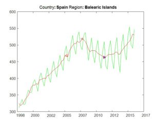
Because of adopting Ron Martin’s methodology for resilience analysis, we had to proceed with the finding of significant peaks and troughs. This was done by the BBQ algorithm (Harding & Pagan, 2002) implemented in the Matlab tool (Engel, 2005). Due to the high variability of the peak position in the immediate vicinity of the economic crisis of 2008, it was necessary to specify a general rule that would suppress this variability. For the needs of analysis, one peak (continued to be marked V) as the beginning of employment downturn due to crisis (2008-2010) and two troughs, one after crisis (we will mark E) and one before the crisis (hereafter D) will be selected from the set of all peaks and troughs. Figure 1 illustrates all of the characteristics described above for the 14th region in Spain (NUTS2 ES53 – Balearic Islands), i.e. the original time series with visible seasonal influences (green), seasonal adjusted series by X13-ARIMA-SEATS (red), (red ), the trough before the crisis (red , in the text marked ) and trough after the crisis (red , in the text marked ).

Fig. 1: Employment in Spain for 14th region (green), smoothened time series (X13-ARIMA-SEATS – red), peak V (red +) and troughs D and E.

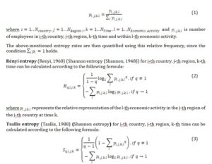
For the purpose of creating explanatory variables, a number of indicators based on several significant definitions of entropy were used. The following will briefly define significant entropy rates.

In the following, the entropy rates are used on employment data to produce the final number of predictors of the impact of the 2008 economic crisis in the EU’s regions. The entropy itself is calculated from the relative frequency of employment in different economic activities in the individual regions of the EU Member States.

The relative frequency (probability) p of employees in a specific quarter and region can be expressed as follows:

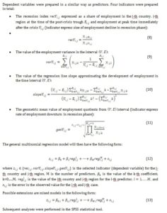
The interval was used instead of the  interval due to a change in the ISIC methodology that caused a sudden change in entropy development. Since the change of methodology was in the immediate vicinity of the peak after the crisis, this change did not cause any significant alternation in quantification of economic changes before the crisis.

Three measures of entropy were specifically selected for further analysis, namely; the Shannon entropy, Rényi entropy (q=2) and Tsallis entropy (q=2). In combination with the indicators defined above, 18 potential predictors were developed, the distribution of which is summarized in Table 2. The set of all predictors will be denoted as .

Table 2: Potential predictors’ distribution and the naming convention

Results

The first step was to select the optimal dependent variable (recY, varY, slopeY or geoY). Due to the large number of predictors, a stepwise method in SPSS Statistics was used to select appropriate dependent variables for the individual dependent variables (other methods generally returned a large number of highly correlated explanatory variables). Table 3 shows the found patterns for the dependent variable recY. Data from all regions was used for the analysis.

Table 3: Model summary of stepwise method for dependent variable recY

1. Predictors: (Constant), Shannon1
2. Predictors: (Constant), Shannon1, Tsallis2

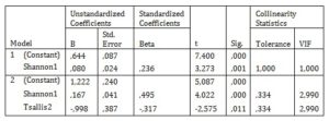
The most suitable predictor in this case is Shannon1, and the Tsallis2 predictor was added for the second model. Table 4 summarizes important information about the coefficients for both selected models. From the VIF values, the Shannon1 and Tsallis2 predictors are relatively strongly correlated (corresponding to a correlation coefficient of 0.81).

Table 4: Coefficients of stepwise models for dependent variable recY

As the second dependent variable, the employment variance (varY) was chosen. However, the stepwise method has not returned any outputs, so it can be concluded that there is no significant predictor in the  set for the employment variance. Therefore, it is possible to exclude it from further analysis.

Another chosen dependent variable is the slope of regression line of employment (slopeY). Table 5 shows that only one significant predictor was found (Shannon0). Table 6 summarizes selected important properties of the coefficients of the model.

Table 5: Model summary of stepwise method for dependent variable slopeY

1. Predictors: (Constant), Shannon0

Table 6: Coefficients of stepwise models for dependent variable slopeY

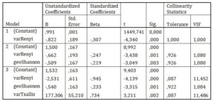
The last dependent variable is the geometric average of the employment shares (geoY). The Stepwise method identified three significant models (see Table 7), whose coefficient of determination is, at first glance, more significant than the previous dependent variables. For this reason, geoY was chosen as the most suited dependent variable in the context of this analysis.

Table 7: Model summary of stepwise method for dependent variable geoY

1. Predictors: (Constant), varRenyi
2. Predictors: (Constant), varRenyi, geoShannon
3. Predictors: (Constant), varRenyi, geoShannon, varTsallis

Table 8 summarizes the selected properties of the coefficients of each model. From the VIF values, the varRenyi and varTsallis predictors in the third model show a high collinearity (correlation coefficient of 0.955), which must be taken into account in further analyses.

Table 8: Coefficients of stepwise models for dependent variable geoY

Potential models for further analysis were Model 2 (the best model without collinearity) and Model 3 (the best model in general). Because the analysed data are naturally hierarchically structured by individual EU member states, it is possible to use the so-called mixed models. For each model, all possible combinations of fixed and random intersections and guidelines were tested, i.e. four options:

• Fixed intercept and fixed slope,
• Random intercepts and fixed slope,
• Fixed intercept and random slopes,
• Random intercepts and random slopes.

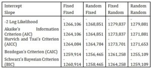
Table 9 illustrates the values of the various information criteria for these four combinations for Model 2. At first glance, it is clear that all criteria positively respond to the addition of random slopes (beta coefficients). For this reason, this model can be called the optimal model in the context of available data and selected indicators without the occurrence of collinearity in explanatory variables.

Table 9: Information Criteria for model 2 (geoY) with dependent variables varRenyi and geoShannon

The information criteria are displayed in smaller-is-better form

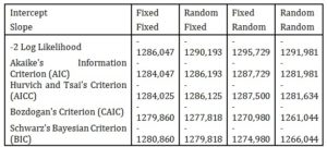
Table 10 presents the information criteria for Model 3. Similar to Model 2, the best results of the model are with random slopes. Only the CAIC and BIC information criteria favour a classical regression model without any influence of particular country.

Table 10: Information Criteria for model 3 with dependent variables varRenyi, geoShannon and varTsallis

The information criteria are displayed in smaller-is-better form.

However, it appears from the results of both models that the influence of the country affects the data, and therefore the use of mixed models is appropriate.

Discussion

Results show that the higher the instability (high varRenyi), the greater the rate of decline of employment in regional recession phase. High varRenyi could mean either growth or decrease or even fluctuation around the average of entropy calculated based on Rényi (q=2). The Adjusted R Squared of the model for dependent variable geoY predicted based on only varRenyi as predictor is about 0,089. Because of this result, this model was enhanced by geoShannon. The results show similar relation like in the case of varRenyi. The more geoShannon grows before the crisis, the higher speed of employment downturn in regional recession phase.

This can be justified by two cases. The growth of entropy could have occurred based on dismissal of employees in sectors that had a large share in the economic activity of the region or, conversely, the growth of entropy is caused by hiring employees in less represented economic sectors. This second interpretation could have been caused by massive subsidies from the European Union before the economic crisis. In both cases, the entropy was increasing in the pre-crisis period.

The predictability of the second model (see table 7) expressed by Adjusted R Square is higher than in the case of the first model (0,129). This improvement of models predictability is because of additional information of Shannon entropy, which is calculated and aggregated during expansion phase before beginning of crisis. However, the third model shows possible collinearity but the predictability is even higher than in the second model (Adjusted R Squared is 0,179). Despite the multi-collinearity issue, the model has good significance for prediction usage. Moreover, mixed model analysis shows the importance of country influence to modelled geoY.

Conclusion

This article gave a new look at the financial crisis in 2008 and discusses the extent to which entropy-based indicators can be useful in predicting regional employment dynamics. The results of the statistical analysis show that while variation of Rényi entropy was high and Shannon’s entropy grew in the pre-crisis recovery phase, the regions showed a higher rate of decline in employment in the subsequent recession. We find also that the Shannon entropy and Tsallis entropy is more suitable for prediction of size of employment downturn (recession index) while the Rényi entropy is the dominant predictor of rate of employment downturn in recession phase. On the other hand, Tsallis entropy plays a different role. The higher the Tsallis entropy measured, the lower the rate of employment in the recession phase. Last part of results show importance of country influence because the information criteria were the lowest in the cases of random slopes in both the second and the third model (for geoY). Results show that the use of entropy, as an indicator in terms of regional policy is a significant predictor of regional resilience. Based on these conclusions, it can be stated that the diversity of economic activities (expressed in terms of entropy measures) presents a significant antecedent to predict the impact of the crisis on a region.

Acknowledges

The paper was supported by the University of Pardubice, Faculty of Economics and Administration, Project SGS_2018_020.

Reference

1. Duit, A., Galaz, V., Eckerberg, K., & Ebbesson, J. (2010). Governance, complexity, and resilience. Global environmental change, 20(3), 363-368.

2. Engel, J. (2005). Business Cycle Dating Programs (BBQ). Retrieved from http://www.ncer.edu.au/resources/data-and-code.php

3. (2017). Labour Force Survey. Retrieved 2016-09-05, from http://ec.europa.eu/eurostat/web/microdata/european-union-labour-force-survey

4. Folke, C., Colding, J., & Berkes, F. (2003). Synthesis: building resilience and adaptive capacity in social-ecological systems. Navigating social-ecological systems: Building resilience for complexity and change, 9(1), 352-387.

5. Harding, D., & Pagan, A. (2002). Dissecting the cycle: a methodological investigation. Journal of Monetary Economics, 49(2), 365-381. doi: http://doi.org/10.1016/S0304-3932(01)00108-8

6. Hill, E., Wial, H., & Wolman, H. (2008). Exploring regional economic resilience: Working Paper, Institute of Urban and Regional Development.

7. Holling, C. S. (1973). Resilience and stability of ecological systems. Annual review of ecology and systematics, 4(1), 1-23.

8. Lengwiler, Y. (2016). X-13 Toolbox for Matlab (Version 1.3). Mathworks File Exchange. Retrieved from https://www.mathworks.com/matlabcentral/fileexchange/49120-x-13-toolbox-for-seasonal-filtering

9. Martin, R. (2012). Regional economic resilience, hysteresis and recessionary shocks. Journal of economic geography, 12(1), 1-32.

10. Martin, R., & Sunley, P. (2007). Complexity thinking and evolutionary economic geography. Journal of economic geography.

11. Martin, R., Sunley, P., Gardiner, B., & Tyler, P. (2016). How regions react to recessions: resilience and the role of economic structure. Regional Studies, 50(4), 561-585.

12. Modica, M., & Reggiani, A. (2015). Spatial economic resilience: overview and perspectives. Networks and Spatial Economics, 15(2), 211-233.

13. Pendall, R., Foster, K. A., & Cowell, M. (2009). Resilience and regions: building understanding of the metaphor. Cambridge Journal of Regions, Economy and Society, rsp028.

14. Perrings, C. (1998). Resilience in the dynamics of economy-environment systems. Environmental and Resource Economics, 11(3-4), 503-520.

15. Pike, A., Dawley, S., & Tomaney, J. (2010). Resilience, adaptation and adaptability. Cambridge Journal of Regions, Economy and Society, rsq001.

16. Reggiani, A., De Graaff, T., & Nijkamp, P. (2002). Resilience: an evolutionary approach to spatial economic systems. Networks and Spatial Economics, 2(2), 211-229.

17. Renyi, A. (1960). On measures of information and entropy. Paper presented at the Proceedings of the 4th Berkeley Symposium on Mathematics, Statistics and Probability.

18. Rose, A. Z. (2009). Economic resilience to disasters CARRI report No. 8: Community and Resilience Institute.

19. Shannon, C. E. (1948). A mathematical theory of communication. Bell System Technical Journal, 27(3), 379-423.

20. Shaw, K. (2012). “Reframing” Resilience: Challenges for Planning Theory and Practice. Planning Theory & Practice, 13(2), 308-312.

21. Simmie, J., & Martin, R. (2010). The economic resilience of regions: towards an evolutionary approach. Cambridge Journal of Regions, Economy and Society, 3(1), 27-43.

22. Tsallis, C. (1988). Possible generalization of Boltzmann-Gibbs statistics. Journal of Statistical Physics, 52(1), 479-487. doi: 10.1007/BF01016429

23. (1989). International Standard Industrial Classification of All Economic Activities, Rev.3.

24. (2008). International Standard Industrial Classification of All Economic Activities (ISIC), Rev.4. New York.

25. Walker, B., Carpenter, S., Anderies, J., Abel, N., Cumming, G., Janssen, M., . . . Pritchard, R. (2002). Resilience management in social-ecological systems: a working hypothesis for a participatory approach. Conservation ecology, 6(1).